Identifying and Predicting the Failure of Valves
Dr. Patrick Bangert
algorithmica technologies GmbH
A chemical plant has a particular unit that is meant to combine several chemicals from a variety of input sources in order to provide a gaseous output (called “tailgas”) with a composition that is as constant as possible.In our particular case, this task is run by an assembly of 40 valves that are controlled by a computer that opens and closes them according to a well-balanced schedule. If the valves do not open and close according to schedule, or if they are either too fast or slow, or if they leak, then the tailgas composition is not constant and causes problems later on in the process. In this study, we demonstrate how to predict future problems and to identify the valves responsible for recurring problems in the composition of the tailgas.
The whole process involves three phases. At the beginning of each phase, some valves are opened or closed to a new position that is then kept for the remainder of that phase. This process repeats forever according to a fixed schedule. For this study, a phase thus means a particular preset degree of openness or closedness for each valve. As the valves have to be mechanically opened and closed at each phase, they age with time and thus respond increasingly poorly to the command to open to a certain degree.
For each of the three phases, we computed the probability distribution of deviations between the set points provided by the control computer, on the one hand, and the actual response as measured by the instrumentation, on the other. The set point is the desired degree of openness for each valve and phase. If, for example, the valve should be open to 70% (set point) and actually is open to 65% (measured), then the deviation is 5%.
If a valve operates normally, we expect the deviation to be almost always very small and, if the deviation is a little larger, we expect it to occur very rarely. In terms of a probability distribution, we expect the curve to start off very high for zero deviation and then to fall off exponentially for higher deviations. This is known as the exponential distribution.
Figure 1 displays the results for each of the three phases. We observe that one phase (the solid line) has an exponential distribution while the two others do not as they have peaks. Seeing secondary peaks (as we observe in the dotted and dashed lines) is not expected as it shows a structured mechanism of deviation and hence some form of damage.
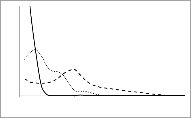
Figure 1: The probability distribution over the three phases of valve operations. The vertical axis is the probability and the horizontal axis the normalized absolute value of the deviation between set point and actual response of valve openings. We observe that one phase appears to be operating correctly (exponential distribution) and two phases incorrectly (non-exponential distributions).
Next, we introduced a measure of abnormality for a valve. The score itself is based on the difference between set point and response (just as in figure 1). However, we also demand that there be an associated surge in non-constancy of the tailgas within a certain response time to track only those abnormal valve openings/closings that were close to an unwanted product surge. In figure 2, we graph the abnormality in this sense for each valve across all three phases of operation.
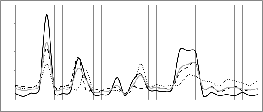
Figure 2: A selection of the 40 valves (horizontal axis) is investigated here in terms of their deviation from the set point (vertical axis) in those cases in which an output pressure surge occurs within a certain time frame. The three black lines correspond to the three phases in figure 1 while the gray line is the average of the three black lines.
Combining these two images, we must look for the dashed and dotted phases in figure 2 and select those valves that have a high score there. We now combine this information with some process specific analysis from the scheduling application (which determines when the valves must open or close). From this we can rule out some valves because they do not open/close in the relevant phase and their deviation is thus a spurious observation. From such an analysis, it is found that only one valve remains. And we attributed the problem to it.
However, while the valve is operating in a way that is not ideal,it is not causing a significant problem just yet. Therefore, let us look over the time evolution of this abnormality in figure 3. The jagged blue line is the abnormality of that one valve at each moment in time. As we are not concerned with the shorter term ups and downs, we take a 20-day moving average to smooth out the curve. This is the thick red line on the plot. We observe an upward trend over time with a dip near the end. We now create a prediction of this time-series, which is plotted in green as the continuation of the red line on the right of the image.
Please note that the peak in the red line of figure 3 is a failure of a valve. After the valve has been fixed, we see the abnormality decline, which suggests that the maintenance measure relieved the problem. However, the abnormality does not decline to its former levels. This means that we have not solved the problem fully. From the prediction made, we predict that another failure is going to occur on the right edge of figure 3. This prediction says that another valve failure will occur in 33 ± 10 days from now.
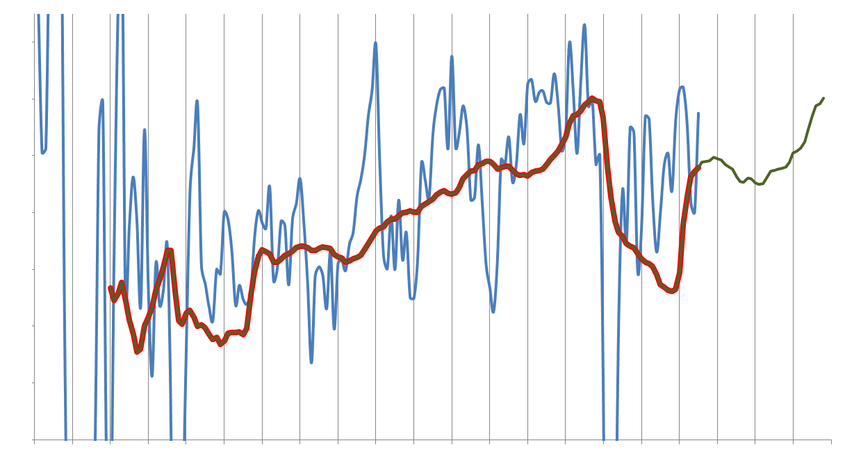
Figure 3: Abnormality over time during the relevant phase together with 20-day moving average and prediction into the future. The peak in the red line is a known failure. The green line represents the predicted evolution. Using the green curve, a prediction is made that another valve failure will occur on the right edge of the plot; this prediction is made 33 ± 10 days in advance. This event occurred as predicted.
After having waited for a few weeks, we found that the failure did indeed happen at the predicted time. The failed valve is the same valve as the one we identified using the above abnormality approach.Thus we conclude that it is possible to predict future valve failures and to identify which valve it will be even if we only have information about the whole family of valves.


